Asymmetric-Key Math

So far, we’ve seen stream ciphers, block ciphers, and hash functions. All those types of algorithm use similar sets of basic operations — addition, rotation, XOR, and other bitwise operations like AND — and they mostly work on bytes and 32-bit integers.

In subsequent chapters, we’re going to look at asymmetric-key algorithms, which are based on a very different style of math. These algorithms generally involve working on very large numbers, hundreds or even thousands of bits long, and doing just a few arithmetic operations on them.

Asymmetric-key algorithms are based on one-way problems. These are computations that are easy to do, but hard to reverse. We will see two one-way problems in this course: one in this chapter, and one in a later chapter.

This area of math is called number theory. In addition, we will look at the basics of the math of elliptic curves. These are the foundation of the newest generation of asymmetric-key algorithms.

Prime Numbers

In number theory, prime numbers are of enormous importance. They are often referred to as just “primes”. A prime number is an integer greater than 1 that is not evenly divisible by any other positive integer, except 1 and itself. The two factors that every number has, 1 and itself, are called its trivial factors; other factors, by contrast, are nontrivial factors.

For example, 2 and 17 are prime. 18 is not prime, because it is evenly divisible by 2, 3, 6, and 9.

The Fundamental Theorem of Arithmetic states that all integers greater than 1 can be expressed uniquely as a product of prime numbers. For example, \(275184 = 2 \cdot 2 \cdot 2 \cdot 2 \cdot 3 \cdot 3 \cdot 3 \cdot 7 \cdot 7 \cdot 13\). There isn’t any other set of prime numbers that you can multiply together to get 275184.

An integer is relatively prime to another one if they have no factors in common other than 1. For example, 21 and 55 are relatively prime to each other, although neither is prime. The term coprime is also sometimes used; it means the same as “relatively prime”.

Groups

A group, in number theory, is a set combined with an operation that takes two members of the set as input, and produces a member of the set as output. A very simple example of a group is the set of integers, and the operation of addition. (The math way to say this is “integers under addition”.)

The set-and-operation combo must have three additional properties in order to be a group:

• Associativity. Informally, this means that rearranging the parentheses in a sequence of many applications of the group’s operation will not change the result. Using integers under addition as an example, this means that the result of \((a + b) + c\) is the same as \(a + (b + c)\).

• Identity element. There must be exactly one member of the set that makes the operation have no effect when used as one input; that member is called the identity element of the group. For example, the identity element of integers under addition is zero, because adding zero to any integer results in that same integer.

• Inverses. Every member of the set must have a corresponding member such that, when the two are used as inputs to the operation, the result is the identity element. For example, the inverse element of \(28\) in the group of integers under addition is \(-28\), because adding \(28\) and \(-28\) together results in zero, the identity element.

This may all seem rather abstract, but group theory is a useful tool for analyzing some cryptographic algorithms, as we’ll see in later chapters.

Group theory is very applicable to modular arithmetic. For example, the integers from 0 to 9 inclusive, with the operation of addition modulo 10, form a group. This is called the additive group modulo 10. The identity element is zero, but it’s important to take a closer look at inverses.

What is the inverse of \(3\) in the additive group modulo 10? It can’t be \(-3\), because that’s not a member of the set: the set here is just the integers from 0 to 9 inclusive. What do you add to \(3\), modulo 10, to get zero? The answer is \(7\), because \(3 + 7 = 10\), and \(10 \Mod 10 = 0\).

Multiplicative Groups

Just as we can define an additive group modulo \(n\), we can also define a multiplicative group modulo \(n\). The identity element is always 1, and we denote the inverse of the element \(a\) as \(a^{-1}\).

There is a very important difference from the additive group: the integer 0 is never included in the group’s set, because 0 has no inverse. Anything multiplied by zero is zero: there’s nothing you can multiply zero by to get any other result. Therefore, it has no inverse, and can’t be included in the group.

Furthermore, the multiplicative group modulo \(n\) only includes the integers from \(1\) to \(n-1\) that are relatively prime to \(n\), because those are the only ones that have inverses. We will sketch the proof later.

For example, let’s consider the multiplicative group modulo 7. Because 7 is prime, all the integers between \(1\) and \(6\) are relatively prime to it, so they are all in the group. What is the inverse element of \(3\)? In other words, what can you multiply \(3\) by so that the result is congruent to \(1\) modulo 7? The answer is \(5\), because \(3 \cdot 5 = 15\), and \(15 \Mod 7 = 1\).

We can check that every element has an inverse: \(1\) is its own inverse, \(2\) and \(4\) are inverses of each other, \(3\) and \(5\) are inverses of each other, and \(6\) is its own inverse.

Let’s look at how this breaks down when the modulus is not prime, and we try to find the inverse of an integer that isn’t relatively prime to the modulus. For example, what if the modulus is 9? The element \(4\) has an inverse, because it is relatively prime to \(9\): the inverse is \(7\), because \(4\cdot 7 = 28\), and \(28 \Mod 9 = 1\). However, what about the element \(6\), which shares a factor with 9? Let’s try multiplying it by every other integer less than 9:

\[\begin{split} 6 \times 1 = 6 & \equiv 6 \pmod{9} \\ 6 \times 2 = 12 & \equiv 3 \pmod{9} \\ 6 \times 3 = 18 & \equiv 0 \pmod{9} \\ 6 \times 4 = 24 & \equiv 6 \pmod{9} \\ 6 \times 5 = 30 & \equiv 3 \pmod{9} \\ 6 \times 6 = 36 & \equiv 0 \pmod{9} \\ 6 \times 7 = 42 & \equiv 6 \pmod{9} \\ 6 \times 8 = 48 & \equiv 3 \pmod{9} \end{split}\]

None of the results are 1, so 6 has no inverse.

In this section, we’ve been finding inverses by hand, trying all the possibilities. In cryptography, we use extremely large moduli (hundreds of digits long) and computing inverses that way is not feasible. Fortunately, there is an efficient algorithm to compute multiplicative inverses, even for extremely large moduli, called the extended Euclidean algorithm.

Modular Exponentiation

Since exponentiation (raising a number to a power) is just repeated multiplication, we can use it in modular arithmetic. We write it the same way as in normal arithmetic. For example, \(3^{11} \equiv 7 \pmod{10}\), because \(3^{11} = 177147\).

It’s worth mentioning modular exponentiation separately, because many asymmetric-key algorithms involve doing modular exponentiation with extremely large numbers, and it may seem unintuitive that this is possible at all, let alone possible within a reasonable amount of time.

For example, imagine computing \(12387161982^{938719287318}\). This is an enormous number: it has about 9 trillion digits. That’s about 30 trillion bits, or 4 terabytes. That’s a lot of storage space, and a lot of computation to fill it all.

What about computing \(12387161982^{938719287318} \Mod 100\)? It turns out that this is considerably easier, and a computer can do it within milliseconds: the answer is 24.

First, we can simply reduce the base modulo 100, because:

\[ (mk + r)^x \equiv r^x \pmod{m},\ r < m \]

We won’t prove this here, but it’s easy to prove by induction on \(x\). This lets us reduce our problem to \(82^{938719287318} \Mod 100\).

Now, recall that \(a^{2x} = (a^x)^2\). This allows us to reduce the modular exponentiation problem to a smaller version of the same problem. We divide the exponent in half, and rewrite the problem as follows:

\[ 82^{938719287318} = (82^{469359643659})^{2} \equiv (82^{469359643659} \Mod 100)^2 \equiv b \pmod{100} \]

Thus, we will instead compute a modular exponentiation with an exponent that is half as large as before. Then all that remains is to square that result, which is less than 100, and reduce the result modulo 100. We can repeat this transformation until the exponent is all the way down to 2. (If the exponent is odd, we will do an extra multiplication.) We’ll have to repeat the transformation roughly \(\log_2(938719287318)\) times, which is about 40.

This algorithm can be slow if the modulus is very large too, as it usually is in asymmetric-key algorithms: 2048 bits is a common modulus size. It is also vulnerable to timing attacks, since it takes different amounts of time based on the exponent (specifically, the number of 1-bits in it). Therefore, in practice, more sophisticated algorithms are used, but we won’t go into them here.

Discrete Logarithms

In normal arithmetic — not modular arithmetic — the logarithm is the inverse operation of exponentiation. If we have \(a^x = b\), then the base-\(a\) logarithm of \(b\) is \(x\). This is written as: \(\log_a(b) = x\).

In words, \(\log_a(b)\) is the answer to the question, “What power do I raise \(a\) to, to get \(b\)?”

In the world of modular arithmetic, there is likewise an inverse to modular exponentiation: the discrete logarithm. It answers the same question as the normal logarithm, but the answer is an integer in the group modulo \(p\). For example, \(3^{11} \equiv 7 \pmod{10}\), therefore we can write \(\log_3(7) = 11 \pmod{10}\).

It is possible for a discrete logarithm not to exist. For example, consider \(\log_2(3) \pmod{10}\). Except for \(2^0 = 1\), there is no power of 2 whose last decimal digit is odd, therefore \(\log_2(3) \pmod{10}\) does not exist.

Computing Discrete Logarithms

As we’ve seen, computing modular exponentiation is relatively easy, even for large moduli and exponents. By contrast, there is no known way to efficiently compute discrete logarithms. As a result, we say that modular exponentiation is a one-way function.

The most obvious way to compute \(\log_a(b) \pmod{m}\) is called trial multiplication: compute \(a \cdot a \Mod m\) and see if it’s equal to \(b\). If not, multiply the result by \(a\) and reduce modulo \(m\) again, and see if it’s equal to \(b\) again. Repeat; count how many times you multiply \(a\) until the result is \(b\), and that count is the value of \(\log_a(b)\).

Trial multiplication is far too inefficient to be useful in computing discrete logarithms on numbers of the size used in cryptography. There are faster algorithms, which we won’t go into here, but none of them fundamentally changes the feasibility of the problem.

There are, however, some special-purpose algorithms that compute discrete logarithms efficiently when the numbers involved have specific mathematical properties. This must be taken into account in discrete-logarithm-based algorithms, as we’ll see later.

Primitive Roots

We must cover one final mathematical concept before we proceed. A primitive root modulo \(n\) is an integer \(g\), such that you can get every number greater than zero, less than \(n\), and relatively prime to \(n\) by raising \(g\) to some power modulo \(n\).

For example, 2 is a primitive root modulo 11:

\begin{align*} 2^1 \Mod 11 &= 2 & 2^6 \Mod 11 &= 9 \\ 2^2 \Mod 11 &= 4 & 2^7 \Mod 11 &= 7 \\ 2^3 \Mod 11 &= 8 & 2^8 \Mod 11 &= 3 \\ 2^4 \Mod 11 &= 5 & 2^9 \Mod 11 &= 6 \\ 2^5 \Mod 11 &= 10 & 2^{10} \Mod 11 &= 1 \end{align*}

By contrast, 3 is not a primitive root modulo 11, because raising it to a power modulo \(n\) only results in five different values:

\begin{align*} 3^1 \Mod 11 &= 3 & 3^6 \Mod 11 &= 3 \\ 3^2 \Mod 11 &= 9 & 3^7 \Mod 11 &= 9 \\ 3^3 \Mod 11 &= 5 & 3^8 \Mod 11 &= 5 \\ 3^4 \Mod 11 &= 4 & 3^9 \Mod 11 &= 4 \\ 3^5 \Mod 11 &= 1 & 3^{10} \Mod 11 &= 1 \end{align*}

Not all moduli have primitive roots. In the algorithms we’re covering in this course, we’ll only be concerned with primitive roots modulo a prime, and prime moduli always have primitive roots.

There is no simple method for finding primitive roots for a given modulus, but it’s not an infeasible problem in the same way that the discrete logarithm is. In practice, primitive roots are found by testing candidates using a slightly time-consuming computation.

Elliptic Curves

The mathematical theory of elliptic curves offers another one-way function that can be used for cryptography, very similar in structure to the discrete logarithm problem. However, the underlying math is very different. We will not look at it in detail here, but just look at the basic idea.

Elliptic curves are equations of the form \(y^2 = x^3 + ax + b\), where \(a\) and \(b\) are constants that define the curve. For example, if we plot the curve \(y^2 = x^3 -2x + 3\) on a graph (so \(a = -2\) and \(b = 3\)), it looks like Fig. 13.

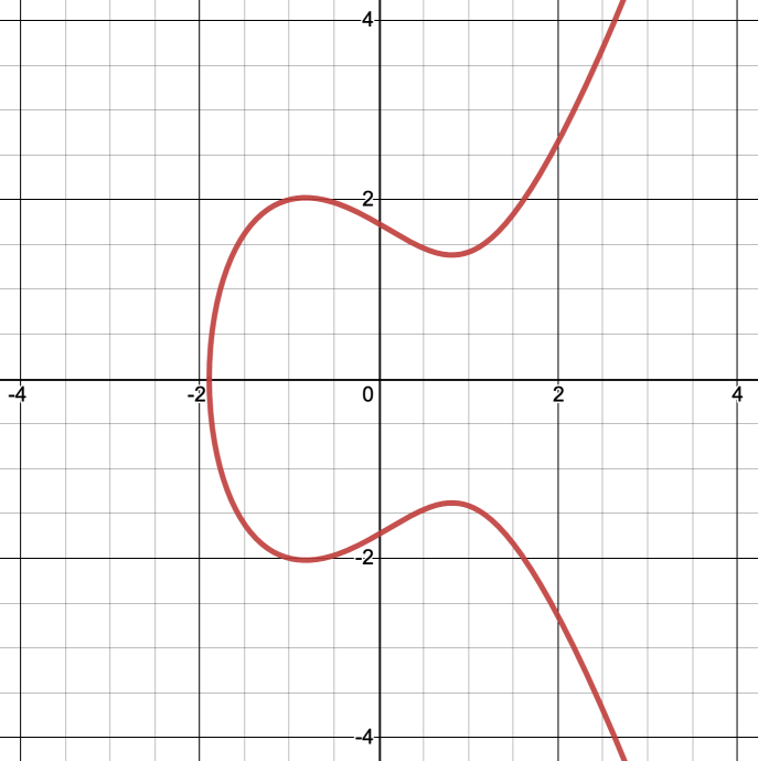
Fig. 13 Part of the elliptic curve \(y^2 = x^3 -2x + 3\). Note that the \(x\)-axis is a line of symmetry.

For cryptography purposes, the important thing about elliptic curves is that if you choose two points on a curve and draw a straight line through them, that line will intersect the curve at exactly one other point. See Fig. 14.

It may seem unintuitive, but unless the line through the two points is exactly vertical, there is always a third intersection point — it may just have very large coordinates if the line is close to vertical ^{1 1}As an example, consider the two points \((-1.7, 1.2194)\) and \((-1.6, -1.4505)\). The \(x\)-coordinates are close together, so the line through them is almost vertical. The third intersection point has coordinates \((716.1597, -19165.2269)\). It exists, but it’s pretty far away.. We’ll address the exactly-vertical case later.

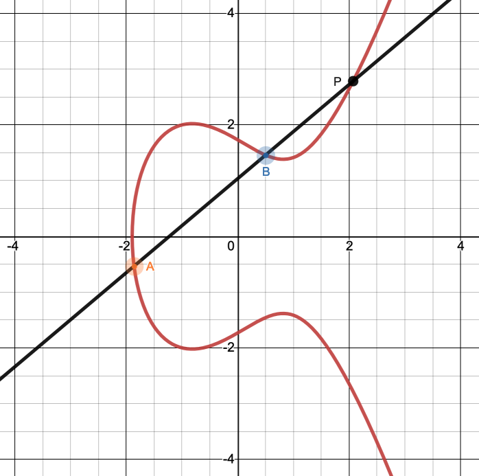
Fig. 14 The line through \(A\) and \(B\) intersects the curve at one other point, \(P\).

This offers us a way to define an operation that combines two points to get a third point. This is called point addition. To add two points \(A\) and \(B\) that are on the curve:

1. Draw a straight line through \(A\) and \(B\). Find the one other point where this line intersects the curve; let’s call that point \(P\). (There is a formula for computing that third point from the coordinates of \(A\) and \(B\), but we won’t go into it here.)

2. Say the coordinates of \(P\) are \((x_P, y_P)\). Then we say that \(A + B = (x_P, -y_P)\). See Fig. 15.

   Note that the \(y\)-coordinate of the resulting point is negated; i.e. it’s the point vertically opposite to \(P\). Because all elliptic curves are symmetric over the \(x\)-axis, negating the \(y\)-coordinate of a point on the curve results in a point that is also on the curve.

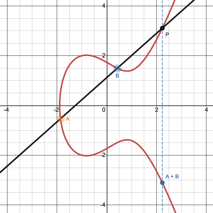
Fig. 15 Elliptic curve point addition: \(A+B\) is the point vertically opposite to \(P\).

There are two special cases in which that procedure for adding points does not quite work. Here are those cases, and how we adapt the definition of addition to account for them.

• If \(A\) and \(B\) are the same point, any line that passes through one passes through both. In this case, the line we draw is the tangent to the curve at that point; there is only one way to draw that. This is also called point doubling. See Fig. 16.

• If \(A\) and \(B\) are vertical to each other, then the line through them does not intersect the curve anywhere else. In this case, we define the result to be a special point at infinity, which is not anywhere on the curve.

  The point at infinity is denoted as \(O\). Furthermore, we define that \(A + O = A\); i.e. adding any point to the point at infinity results in just that same point.

Fig. 16 To add a point \(A\) to itself, draw the tangent to the curve at \(A\).

We won’t go into the details here, but there are very simple formulas for computing point addition and point doubling.

Elliptic-curve point addition forms a group. It has all the necessary properties:

• Associativity: \((A + B) + C\) is the same as \(A + (B + C)\). The proof of this is quite complex, so we won’t go into it here.

• Identity element: the point at infinity, \(O\), is the identity element, because \(A + O = A\).

• Inverse elements: the inverse of the point \((x, y)\) is the point \((x, -y)\), because adding those two points together results in the identity element \(O\).

Furthermore, it is commutative: \(A + B\) is the same as \(B + A\).

Now that we’ve defined an addition operation, we can define multiplication, since multiplication is just repeated addition. We define scalar multiplication of a point \(P\) by a number \(n\), to be \(P\) added to itself \(n\) times. For example, \(4 \cdot P = P + P + P + P\).

Because point addition is associative, that calculation can be done with only two additions instead of three. First, compute \(Q \leftarrow P + P\), then compute \(Q + Q\). In general, this works much like modular exponentiation: to compute \(2n \cdot P\), first compute \(n \cdot P\), then double the resulting point.

This gives us the basis of a one-way function. It is relatively easy to compute \(n \cdot P\) even for very large values of \(n\). By contrast, given only \(P\) and \(n\cdot P\), there is no known way to efficiently compute \(n\). This is called the elliptic-curve discrete logarithm problem ^{2 2}This is a bit of a misnomer, because a logarithm is the inverse of exponentiation, not multiplication. But we’re stuck with it..

In Cryptography

The above is just to give you an intuition for elliptic-curve operations; it is not what’s actually done in elliptic-curve cryptography.

In what we’ve seen so far, we’ve been working with points on the curve with coordinates that are real numbers; i.e. they can have fractional parts, and be of any size. In cryptography, we restrict the points to having coordinates that are integers modulo some prime number \(p\), and take the elliptic curve equation to be a congruence modulo \(p\) instead. This is an elliptic curve over a finite field:

\[y^2 \equiv x^3 + ax + b \pmod{p}\]

For example, let’s look at the same curve we looked at above, but modulo the prime number 61:

\[y^2 \equiv x^3 - 2x + 3 \pmod{61}\]

For example, the point \((5, 22)\) is on this curve, because \(22^2 \Mod 61 = 57\), and \((5^3 - 2(5) + 3) \Mod 61 = 57\). Fig. 17 is a plot of all the points that satisfy that congruence.

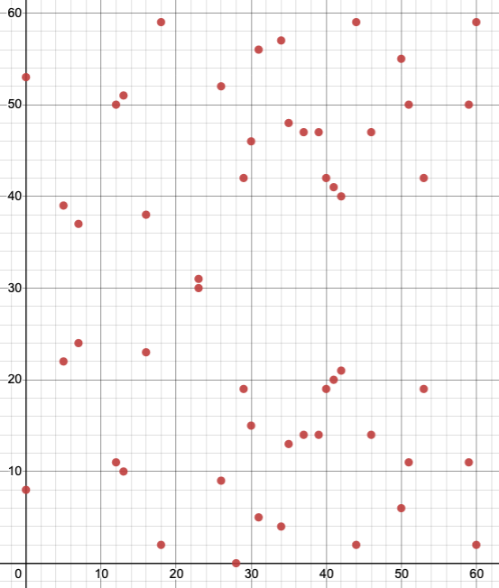
Fig. 17 The points of \(y^2 \equiv x^3 - 2x + 3 \pmod{61}\).

We still call this a “curve” even though it’s just a bunch of scattered points. One important thing to note is that there is still a horizontal line of symmetry: every point has a corresponding point with the same \(x\)-coordinate and a \(y\)-coordinate that is its additive inverse modulo 61. For example, the point \((5,22)\) has the corresponding point \((5,39)\), because \(22 + 39 \Mod 61 = 0\).

The formulas for computing point addition and point doubling on finite-field elliptic curves are almost the same as on real-number curves. The only difference is that instead of doing division, as the real-number formulas do, the finite-field formulas multiply by a modular multiplicative inverse.

Furthermore, scalar multiplication on finite-field curves has the same one-way property as scalar multiplication on real-number curves. It’s easy to compute \(n \cdot P\) from \(n\) and \(P\), but hard to compute \(n\) from \(P\) and \(n\cdot P\). This problem is the basis of elliptic-curve cryptography.

One important concept in finite-field curves that has no equivalent in real-number curves is the order of a point. If you compute \(n \cdot P\) for larger and larger \(n\), you will eventually get \(O\) as the result. (This is not obvious, but we’ll skip the proof here.) The value of \(n\) such that \(n \cdot P = O\) is called the order of \(P\).

The elliptic-curve algorithms we’ll look at involve the choice of a specific point, the base point, on which to do computations. The order of the base point determines how many possible private keys there are, and thus determines the curve’s security level.

Because of the nature of elliptic curve math, orders of points don’t generally line up nicely on powers of two. (E.g. one popular curve has a fixed base point whose order is approximately \(2^{252}\).) Orders of around \(2^{256}\) are considered secure, providing security approximately equivalent to a symmetric-key cipher with a 128-bit key.

We’ve so far only looked at curves over prime fields (i.e. modulo a prime number), but there is another type of curve used in cryptography: those over binary fields. These use the same Galois multiplication that we saw in AES (in the MixColumns step) and in Galois/Counter mode. The computations for point addition and multiplication in binary fields are different, but the overall structure is similar to that in prime fields. Prime fields, however, are better studied, and considered more secure.

Other Equation Types

The type of curve equation we’ve been looking at, \(y^2 = x^3 + ax + b\), is called a Weierstrass curve. There are other types of curve equations; the ones you’ll sometimes hear about in cryptographic contexts are:

• Montgomery curves: \(by^2 = x^3 + ax^2 + x\)

• Twisted Edwards curves: \(ax^2 + y^2 = 1 + d x^2 y^2\)

These alternative curve equation types have different formulas for computing point addition and doubling on them, and these different formulas can offer security and performance benefits. For example, in Montgomery curves, computing the \(x\) coordinate of added or doubled points only involves the \(x\) coordinates of the input point, not the \(y\) coordinates. This means that \(y\) coordinates can be omitted altogether.

Furthermore, some curve types make it easier to implement scalar multiplication without allowing timing attacks that could reveal the value of the scalar. This is important since elliptic-curve algorithms generally use a secret value as the scalar.

Named Curves

Algorithms that use elliptic curves require you to choose a specific curve, and a point on the curve; these choices are collectively called parameters. Parameter choice is very consequential. Poor choices of curve or base point can result in degraded security or performance. To complicate matters, it is generally not easy to look at a curve equation or base point and determine whether it is a good choice.

Therefore, essentially all real-world implementations of elliptic-curve cryptography use pre-made sets of parameters to mitigate these problems. These pre-made parameter sets are called named curves. Note that named curves include a base point, not just the curve equation.

Various organizations have published named curves. Here are some of the common ones, all of which are Weierstrass curves:

• The Standards for Efficient Cryptography Group (SECG) defines curves with names like secp192r1, secp224k1, sect163r1, and sect163r2, among many others.

• NIST defines curves with names like P-256, K-283, and B-571.

• ANSI X9.62 defines curves with names like prime256v1 and c2tnb239v1.

• Brainpool curves, published in RFC 5639.

There is some overlap between the curves that different organizations standardize. For example, what SECG calls secp256r1, NIST calls P-256, and ANSI calls prime256v1 are all the same curve.

The three-digit numbers in the curve names refer to the bit length of the order of the base point; e.g. P-256’s base point has order \(2^{256}\). Elliptic curves provide security roughly equivalent to a symmetric key of half that length.

Some of these named curves come with detailed descriptions of how they were generated. It is very notable, though, that some of the popular NIST curves do not, such as P-256. (The parameters were generated using a hash function, but there is no explanation for the input to the hash function.) It is known that the NSA was involved in creating the NIST curves, and the open cryptographic community suspects that the NSA weakened the curves in a way that they can exploit. Some cryptographers recommend avoiding the NIST curves altogether. (This kind of suspicion is why nothing-up-my-sleeve numbers are favored when random-looking constants are needed in algorithms.)

Another notable named curve is Curve25519, a Montgomery curve. It was designed by Daniel Bernstein ^{3 3}The same person who designed ChaCha20 and Poly1305. It’s an interesting phenomenon that the latest generation of cryptographic standards is converging on a suite of algorithms that are all designed by one guy.. It has a very minimalistic, nothing-up-my-sleeve definition, and some pleasing mathematical properties, making it a favorite among cryptographers. Its base point is \(x=9\), and has order \(2^{252}\).

Daniel Bernstein and Tanja Lange have published a project called SafeCurves[BL], in which they evaluate many named curves in terms of things like how suspicious their origins are, how fast their implementations can be, and how easy they are to implement without side channels. They recommend a few named curves, one of which is Curve25519.

Caution

Never use any elliptic-curve algorithm with something other than a named curve. Many implementations don’t even support non-named curves, so this is unlikely to be an issue, but be warned anyway.

See Also

• The website I used to create the graphs of elliptic curves. It allows you to dynamically adjust the curve and compute intersection points. This link includes filled-out formulas for point addition; you can move the points around to see the result of adding them.

• An interactive EC point addition/multiplication tool. Supports both real-number and finite-field curves.

Key Takeaways

• A prime number is an integer that is not divisible by any integer except 1 and itself.

• A group, in the mathematical sense, is a set plus an operation that combines two elements of the set and produces a third. Group theory is useful in analyzing how modular arithmetic works.

• It is easy to raise a number to very large powers under a modulus, but infeasible to do the opposite (compute what power a number was raised to under a modulus, to get a certain result). This is the discrete logarithm problem.

• Elliptic-curve math contains a problem very similar in structure to the discrete logarithm problem.

• Algorithms that use elliptic curves should always use pre-made curves and points, to avoid security and performance problems. These pre-made values are called named curves.

---